In political science ideal points are the most common measure describing judges’ votes.  The goal of ideal points in the study of courts is locating the relative political ideology of a judge on a scale of liberal to conservative.  Of course what it actually means to be a conservative or liberal judge is somewhat contested.

For the Supreme Court the common ideal point metric is a Justice’s Martin Quinn Score (2002). Without going into the specifics of generating ideal points (I’ll deal with that in another post), one way is based on coding a Justice’s votes from prior terms.  This coding of votes is typically based on information aggregated in the Supreme Court Database.  An important aspect of ideal point generation is that it scales a Justice’s policy position relative to the other Justices.

Social network analysis provides another means to describe a Justice’s voting patterns.  In the example in this post I located the Justices’ voting patterns for OT 2014.  Rather than scaling the Justices’ votes on an ideological scale, the tools of network analysis allow us to understand the magnitude of a Justice’s voting power on the Court.  A good explanation and example are provided in a blog piece here.

To generate the network I took all of the Justices’ votes for the Term (from the Supreme Court Database) and located all co-occurrences – when Justices voted in the same direction in a case.  I used these percentages of agreements as weights for each pair of Justices’ relationships so that there was a percentage for every possible Justice pairing.  The final product was a list of each Justice pairing with the associated weight of their relationship (since there is no direction in the weight of the relationship this network is known as “undirected”).

With these weights, I constructed a network graph using the visualization program Gephi found below.

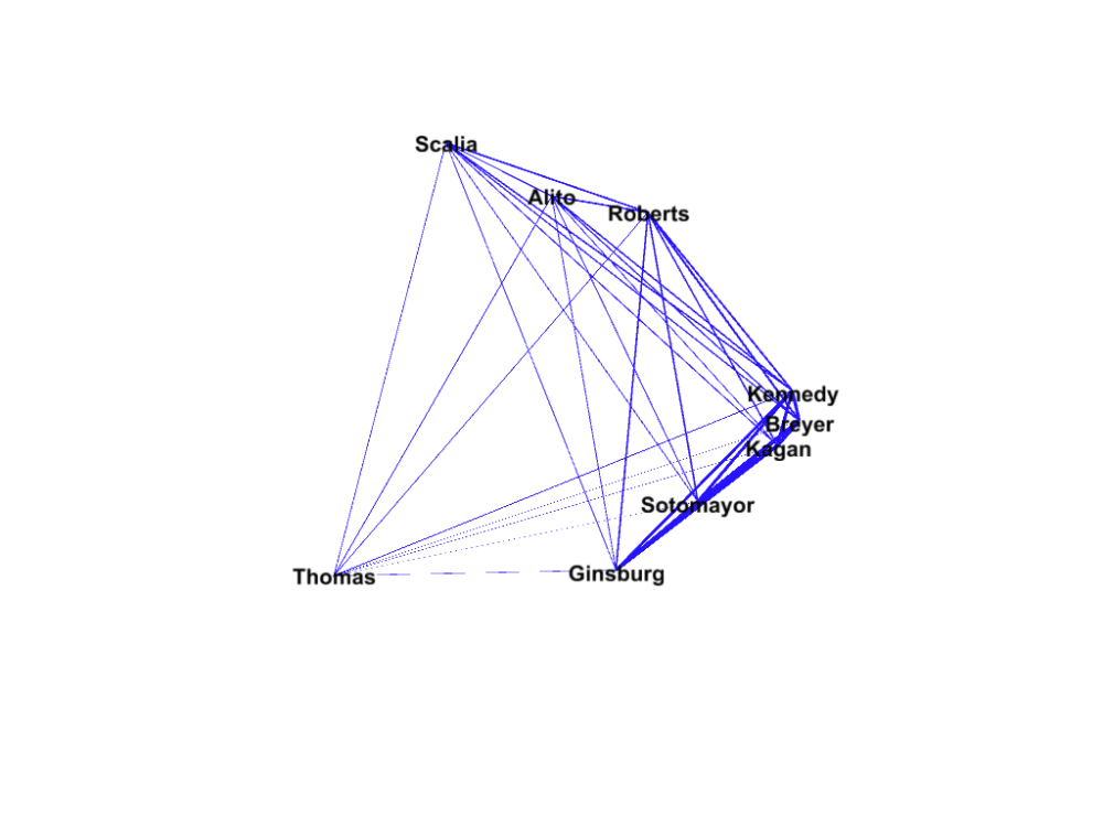
The thickness of the lines relate to the strength of the relationship between any Justice pair.  As is evident from the graph the Justices have a varying number of strong and weak ties.

I then calculated  the Justices’ centralities in the network.  While Gephi provides nice visualizations of network graphs I prefer the tools for calculating network attributes in R.  I imported the list of justice-pair weights into R with the igraph package to calculated each Justice’s centrality.  This essentially gives a sense of a Justice’s connectedness within the entire network (I used the eigenvector centrality measure which is described in greater depth here).

The Justices’ centralities for OT 2014 are:

Scalia 0.8

Kennedy 0.97

Thomas 0.7

Ginsburg 0.96

Breyer 1.0

Roberts 0.87

Alito 0.8

Sotomayor 0.96

Kagan 0.97

Possibly surprisingly given the rhetoric of the current Court, the “liberal” justices were much more central in the voting in OT 2014 according to this metric than the “conservative” justices.  While the Justice often touted as the Court’s median, Justice Kennedy, was the second most central justice, Justice Breyer was the most central.  While this does not show that Justice Breyer was a tie-breaking vote in 5-4 decisions in the same manner as Justice Kennedy, this does show that Justice Breyer was often a central component of voting coalitions on the 2014 Court (which is somewhat surprising given the lack of scholarly and media-related attention paid to Justice Breyer relative to many of the other Justices).

There are many other uses of social network graphs for studying courts.  In this case they provide an interesting way to visualize and compute a Justice’s voting power and some novel insights into the Justices’ votes.